Data Tables
Data for this project was organized into 2 data tables, Table 3 shows a subset of site information as well as the normalized values of organic carbon parameters collected. Table 4 shows a subset of ASV raw counts/sample obtained using the QUIIME2 bioinformatic pipeline.
Table 3: Example values of unnormalized organic carbon parameters and site information for the first five 2019 samples. ID was the unique identifier given for each sample, name refers to the site name. Distance range was assigned as near (<7km), mid (18-25km) and far (>35km). Latitude and longitude are the coordinates for the site location. Glacier refers to the glacier that feeds the associated river, river refers to the river that was sampled, and date is the date sampled. dC14 and d13C are carbon isotope values (%o). A254 (m-1), S275-295(m-1) and SUVA (m-1) are absorbance parameter values.

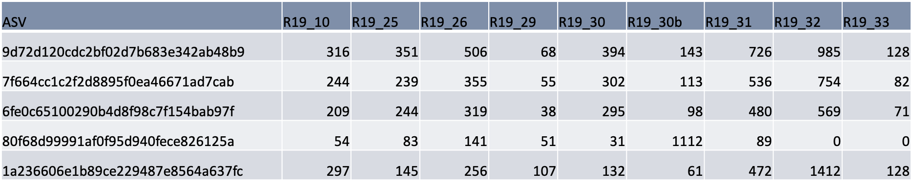
Table 4: The first five rows in the ASV data table showing raw count values (the number of times that ASV was present in the sample) associated with unique ASVs for a subset of 2019 samples. Each ASV represents a unique microbial species/group.
Outlier Removal
Carbon Parameters
Scatterplots: DOC, A254, S275_295 and SUVA was plotted as scatterplots against each other (Figures 5). From these plots samples R19_16-R19_24 were classified as DOC outliers since they deviate from the highly linear established relationship between DOC and A254 (Figure 5).
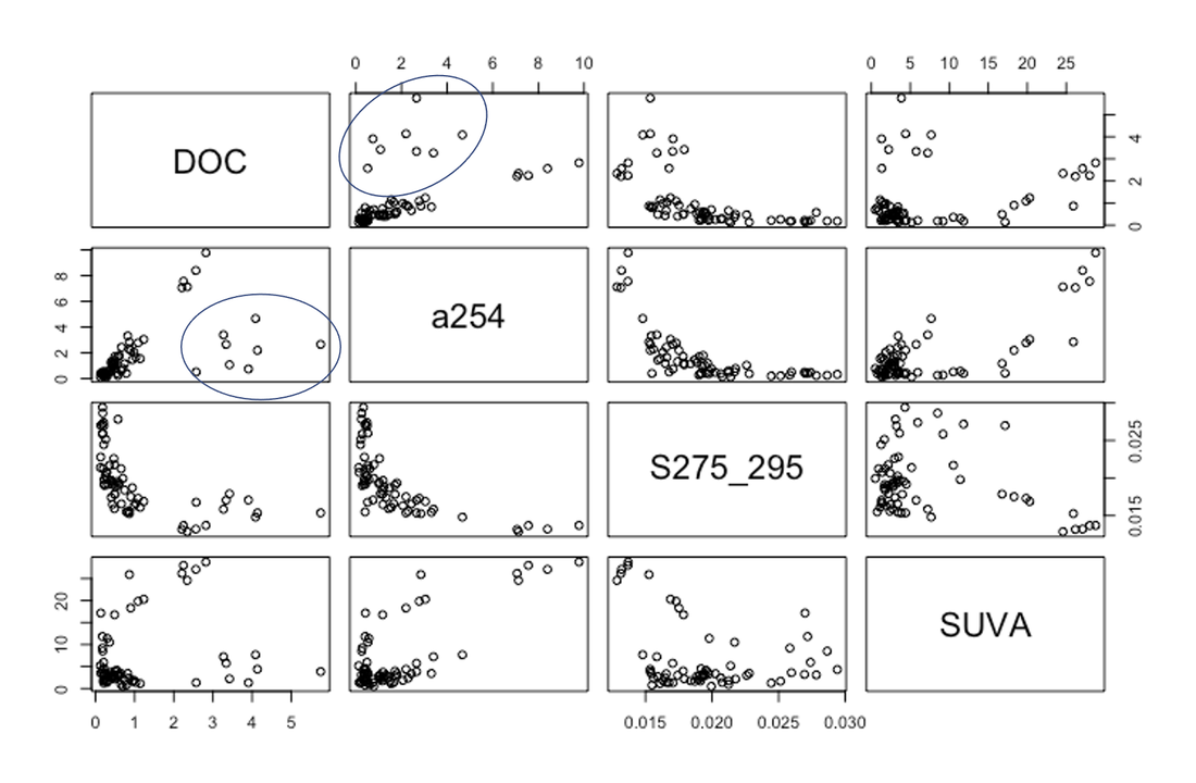
Figure 5: Scatterplots of different combinations of unnormalized organic carbon parameter values. Samples circled in blue represent samples R19_16-R19_24 and were classified as outliers and removed from further analysis. DOC (ppm), A254(m-1), S275-295 (m-1), SUVA (m-1).
Timeseries: Time series were plotted for all organic carbon parameters, with the DOC outliers still removed (Figures 6 A-F). No outliers were identified from these plots.

|

|

|

|

|

|
Figure 6: Time series of (A) A254 (m-1) (proxy for humic components) (B) S275-295 (m-1) (proxy for low molecular weight) (C) DOC (ppm) (amount of organic carbon) (D) SUVA (m-1) (proxy for aromaticity) (E) delta13C (%0) (terrestrial carbon tracer) and (F) delta14C (%0) (proxy for carbon pool age).
Microbial Samples
A bar plot was made to investigate the total ASV count per sample (Figure 7). From this samples R19_33, R19_51 and R19_60 were identified as outliers due to their low total ASV count and were removed from further analysis.
A bar plot was made to investigate the total ASV count per sample (Figure 7). From this samples R19_33, R19_51 and R19_60 were identified as outliers due to their low total ASV count and were removed from further analysis.
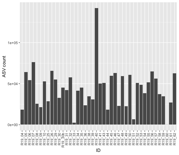
Figure 7: Bar plot showing the total ASV count per sample
Data Normalization
Organic Carbon
Histograms were conducted for each organic carbon parameter to assess normality (Figures 8 A-I). DOC, S275-295, SUVA, and A254 were identified as being skewed and were log transformed for continued analysis to achieve a more normal distribution.


|


|

|

|
Figure 8: Histogram of (A) DOC (ppm) (amount of organic carbon) (B) log transformed DOC (C) SUVA (proxy for aromatic components) (D) log transformed SUVA (E) S275-295 (proxy for low molecular weight) (F) log S275-295 (G) A254 (proxy for humic components) (H) log transformed A254 (I) delta13C (tracer for terrestrial carbon (J) deltaC14 (carbon pool age)
Microbial Samples
A histogram was conducted on raw count ASV data (Figure 9A) to assess normality. The histogram was determined to be skewed therefore a hellinger transformation was conducted on the raw count data (Figure 9B) to achieve a more normal distribution.
A histogram was conducted on raw count ASV data (Figure 9A) to assess normality. The histogram was determined to be skewed therefore a hellinger transformation was conducted on the raw count data (Figure 9B) to achieve a more normal distribution.

|

|
Figure 9: Histogram of (A) total unnormalized ASV count and (B) hellinger transformed ASV count
