Field Sampling
Site Information
Samples for organic carbon and microbial community composition were collected in 2019 from four glacier-fed rivers located within Banff and Jasper National Parks: the Athabasca River, Sunwapta River, North Saskatchewan River, and Bow River (Figure 2). In total fourteen sites were selected ranging from 0-100km downstream with each site having at least one near (site<10km), mid (15km<site<25km) and far (site >35km) site relative to glacial headwaters. This distance gradient was chosen to explore how microbial communities and organic carbon pools change with increasing distance away from glacier. Each site was sampled monthly from May-October 2019. The purpose of the monthly sampling design is to compare carbon pool characteristics and microbial communities communities at times with different hydrological inputs into the streams from predominately snowmelt inputs (May and June) to glacial melt inputs (July-October) (Figure 3).
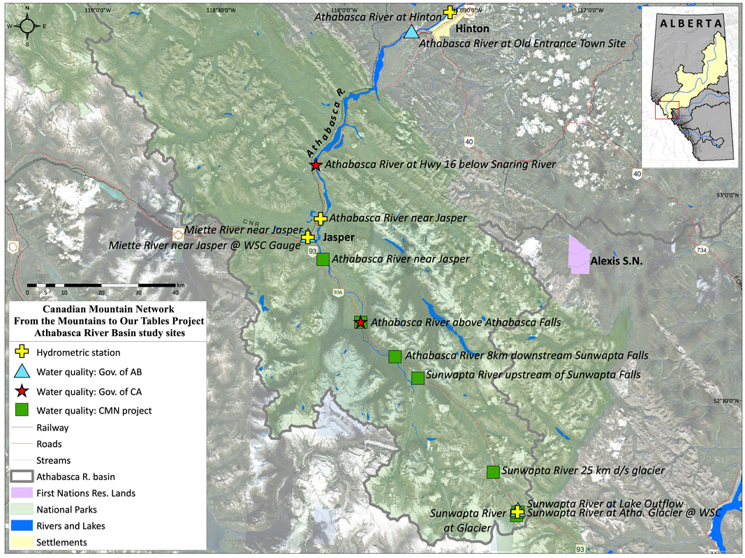
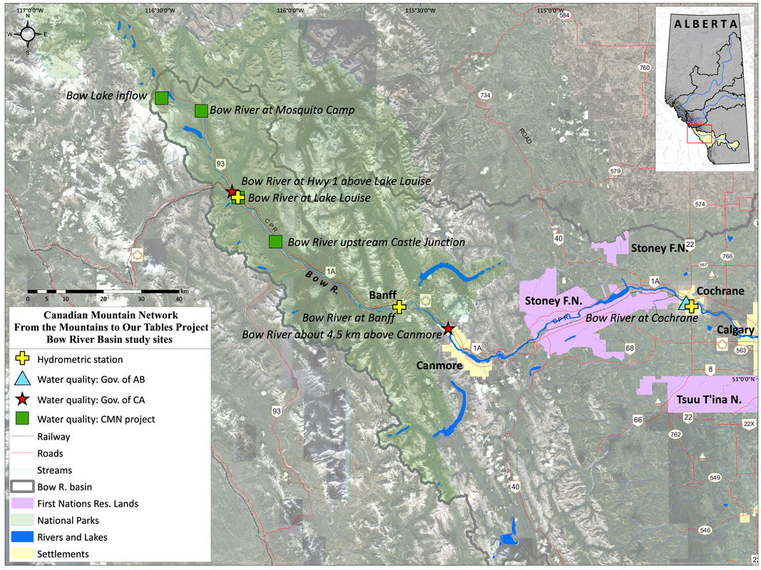
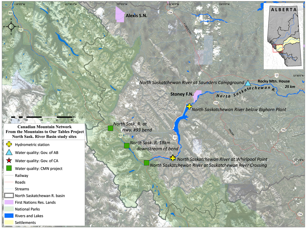
Figure 2: Study site locations for Athabasca and Sunwapta River (top), Bow River (middle) and North Saskatchewan River (bottom). Maps created by Craig Emmerton.
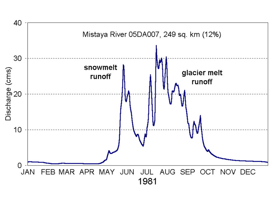
Figure 3: Representation of a typical glacial hydrograph in the Canadian Rockies showing the changing stream inputs throughout a year (18).
Field Sample Collection
Parameters: Parameters collected to characterize the organic carbon pool were dissolved organic carbon (DOC), absorbance (to calculate absorbance parameters A254, SUVA254 (SUVA), and S275-295), delta13C (d13C), and delta14C (d14C). What each of these parameters are able to indicate about the organic carbon pool characteristics are summarized in Table 2. Samples were also collected for 16s rRNA gene sequencing (box 3) for microbial community analysis.
Parameters: Parameters collected to characterize the organic carbon pool were dissolved organic carbon (DOC), absorbance (to calculate absorbance parameters A254, SUVA254 (SUVA), and S275-295), delta13C (d13C), and delta14C (d14C). What each of these parameters are able to indicate about the organic carbon pool characteristics are summarized in Table 2. Samples were also collected for 16s rRNA gene sequencing (box 3) for microbial community analysis.
- Absorbance, DOC, delta13C: For each parameter, water was collected on site and 0.45µm filtered into combusted amber glass EPA vials using sterile polyethersulfone (PES) filters (Figure 4 A). DOC and 13C samples were preserved to pH 2 using 10% hydrochloric acid within 24 hours. All samples were stored at 4°C until analysis.
- delta14C: Samples were collected as bulk water at site using acid washed 2L teflon bottles, then vacuum filtered using a combusted glass setup through 0.7µm combusted glass microfiber filters (GF/F) within 24 hours (Figure 4B). Filtrate was collected into combusted amber 1L glass bottles and acidified to pH of 2 using HPLC grade phosphoric acid for preservation, then stored 4°C until analysis.
- Microbial community: Samples were collected at site using autoclaved 4L polycarbonate bottles. At the field lab water samples were filtered within 24 hours using a peristaltic pump and a sterile 0.2µm Sterivex filter (Figure 4C). Sterivex filters were stored at -80°C until analysis.
Table 2: Table summarizing the organic carbon parameters collected and what aspect of the carbon pool these parameters are used to characterize.
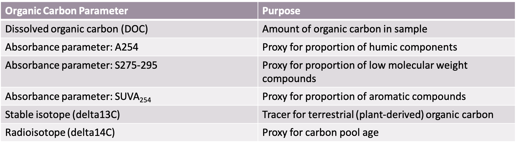
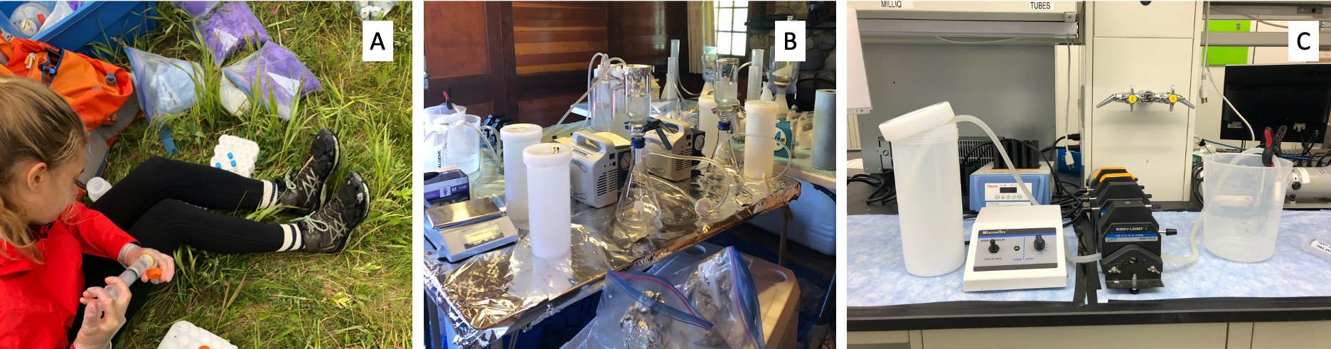
Figure 4: Filtration set up used for (A) hand filtering for absorbance, DOC, and delta13C, (B) vacuum filtration for delta14C ,(C) peristaltic filtering for microbial community analysis
Lab Analysis
- Absorbance: Samples were run on a Horbia Aqualog spectrophotometer to provide absorbance spectra. Spectra was used to calculate A254 (proxy for proportion of humic material), S275-S274 (proxy for molecular weight), and SUVA (proxy for aromaticity) (9).
- DOC: Samples were run on a Shimadzu total organic carbon analyzer, providing concentrations.
- delta13C: Samples were sent to the Environmental Isotopes lab at the University of Waterloo to be run on an isotope ratio mass spectrometer (IRMS) providing delta13C values (tracer for terrestrial carbon)
- delta14C: Samples were sent to the A.E Lalonde lab at the University of Ottawa and ran on an accelerator mass spectrometer to provide relative age of organic carbon pool (delta14C)
- Microbial community analysis: DNA was extracted from Sterivex filters using Quigen DNeasy Power Water kit. Samples were then amplified using PCR targeting the v4-v5 hyper-variable region of the 16s rRNA gene (20). The amplified product was sequenced utilizing high throughput sequencing techniques on an Illumina MiSeq sequencer. Raw data processed using the Quantitative Insights Into Microbial Ecology (QUIIME2) bioinformatic pipeline to give counts of amplicon sequence variants (ASV) present in the sample (box 4).
|
Box 3: 16s rRNA Gene Sequencing The 16s rRNA gene is present in almost all bacteria. It contains sections that are highly conserved, and sections that are hyper-variable. DNA sequencing of certain hyper-variable sections within this gene can be used to taxonomically identify unique species of bacteria. |
Box 4: Amplicon Sequence Variants An amplicon sequence variant (ASV) is a unique and corrected DNA sequence obtained from 16s rRNA gene sequencing. Each ASV can be thought of as a unique microbial species/group. Taxonomic information is assigned to ASVs through databases such as the SILVA database. |
Data Analysis
All data analysis was run in R Studio (version 1.2.5042)
Objective 1: Carbon parameters (A254, DOC, SUVA, S275-S295, d13C and d14C) were first plotted as scatter plots and time series to check for outliers (see data page). Next, histograms were plotted to visually assess the shape of the distribution (see data page). A254, DOC, SUVA, and S275-295 were log transformed to achieve more normalized distributions. Throughout analysis carbon parameters were analyzed as three different groups: (1) A254, DOC, SUVA, S275-S295, (B) A254, DOC, SUVA, S275-S295, d13C, and (3) A254, DOC, SUVA, S275-S295, d14C. This was done due to d13C and d14C values only being collected at a small subset of sites, and not both at the same site. This was due to a sample collection error, and future field seasons will collect d13C and d14C at every site.
Carbon parameters were initially visualized using a principal component analysis (PCA) to visually assess if month, river, and proximity to glacier led to a separation between sample points, and by what parameters (see data exploration page). A PCA is a rotation-based technique where points are rotated in a way that shows the most variation between the points (see data exploration) (19). Alternatively, carbon parameters could have been visualized utilizing distance-based techniques such as non-metric multidimensional scaling (NMDS), or principal coordinate analysis (PCoA), however the PCA gave the best representation of the variance between my groups of interest (river, distance from glacier, and month sampled).
After data exploration a discriminant analysis was performed to assess changes in organic carbon parameters based on distance from glacier, month sampled, and river sampled (see results and discussion page). A linear discriminant analysis is similar to a PCA, but it shows that maximum variation between groups rather than the variation between all points (19). This method was selected as it best answered my objectives and still represented a lot of variation within my dataset. The purpose of the discriminant analysis was to visually assess which organic carbon parameters were associated with my different groups (month, river, proximity to glacier). This analysis was followed up with a multivariate analysis of variance (MANOVA). A MANOVA is an extension of ANOVA, testing whether grouping variables can explain variation in multiple response variables (19). The purpose of the MANOVA was to determine if any of my groups (month, river, proximity to glacier) were significantly different. A MANOVA was chosen over distance-based techniques such as multi-response permutation procedure (MRPP) or permutational MANOVA (perMANOVA), as it best complimented the discriminant analysis (a rotation-based technique). The MANOVA was followed up utilizing pairwise comparisons (Holms-Sidak correction) and univariate analysis (ANOVA). Pairwise comparisons were utilized to assess which groups were significantly different from each other, and univariate analysis was used to determine which carbon parameters were significantly varying with my different groups (month, river, proximity to glacier). PCA, discriminant analysis, MANOVA, and ANOVA all assume normally distributed data, which is why highly skewed data were normalized before analysis.
Objective 2: Microbial sequence data (ASV count data) were checked for outliers, and samples that had relatively less total ASV counts were removed (see data page). Next, the microbial data was Hellinger transformed (see data page). The Hellinger transformation is a common transformation used on microbial species data, and it accounts for the presence of zeros within the dataset (19). To visualize changes in microbial communities an NMDS was performed on Bray Curtis distance matrix on normalized ASV data (see data exploration page). An NMDS is an ordination on a distance/dissimilarity matrix to graphically represent the minimum dissimilarity between sample points (19). A distance-based ordination was chosen over a rotation-based metric (such as PCA) because the ASV data was highly zero inflated, and the use of a distance-based technique allowed for the use of the Bray Curtis distances which are able to handle highly zero inflated species datasets. An NMDS was selected over PCOA (another distance-based ordination) because they resulted in a similar plot, and the NMDS is more commonly used in the field. The purpose of the NMDS plots were to visually assess if there was a separation of sample points by my groups of interest (month, river, proximity to glacier). The NMDS plots were followed up with a perMANOVA. A perMANOVA is similar to a MANOVA but it utilizes distance matrices (19). The purpose of the perMANOVA was to assess if my different groups (month, river, and proximity to glacier) led to a significant difference in microbial communities. PerMANOVA does not assume normal distributions, like MANOVA which is why is was chosen for this analysis. Assumptions of perMANOVA are that samples are independent from each other (19). PerMANOVA was then followed up with pairwise testing (pairwise perMANOVA) to assess differences between groups.
Objective 3: To investigate how organic carbon parameters (A254, DOC, S275-295 and SUVA) may lead to variation in the microbial community composition a distance-based redundancy analysis was performed utilizing a bray Curtis distance matrix of Hellinger transformed microbial community data, organic carbon parameters and sampling information (month, distance and proximity to glacier). A redundancy analysis is a constrained gradient analysis that examines how the variation in a response dataset (in this case microbial community) can be explained by a set of predictor variables (in this case organic carbon parameters and sampling information) (19). A distance-based redundancy analysis performs a redundancy analysis on a non – Euclidean distance matrix. A distance-based redundancy analysis was chosen over a redundancy analysis, canonical correspondence analysis and other constrained gradient techniques because it allowed for the input to be a non-euclidean distance matrix. The use of a non-euclidean distance matrix was important for this dataset, as it was highly zero inflated and the Bray-Curtis distance matrix corrects for this. Distance based redundancy analysis assumes that the number of explanatory variables is less than the number of samples (which is why d13C and d14C were not included in this analysis), and that the explanatory variables are normalized and scaled (19).
